The code was updated on February 27, 2026.
Advances in Machine Learning and Their Application to Materials Science

Machine learning is rapidly transforming materials science, shifting the field from a traditional trial-and-error approach to a more predictive and accelerated paradigm of materials discovery and design. This evolution is driven by the growing availability of large materials databases, increased computational power, and the development of sophisticated machine learning algorithms capable of uncovering complex relationships between a material's structure and its properties. Current developments focus on using machine learning for rapid screening of candidate materials, predicting their performance, and even generating novel materials with desired characteristics. For instance, machine learning models are being employed to discover new materials for solar panels by predicting how structural changes will affect their efficiency in converting sunlight to electricity.
A significant area of progress lies in the application of advanced AI techniques to solve fundamental challenges in materials science. Researchers at Caltech, for example, have recently developed an AI-based method to dramatically speed up complex calculations of quantum interactions, such as those among atomic vibrations (phonons), which are critical for determining a material's thermal properties. This approach uses machine learning to compress the enormous tensors that describe these interactions, reducing computational complexity by orders of magnitude without sacrificing accuracy. Furthermore, the integration of machine learning is poised to enhance every stage of the scientific process, from generating hypotheses and planning experiments to analyzing results, fostering a human-machine partnership that promises to accelerate research at an unprecedented rate. This data-driven approach is significantly reducing the cost, risk, and time associated with materials research and development.
An Introduction to the Most Advanced Models in Materials Science
1. Generative Models for Inverse Design
Inverse design is a paradigm shift in materials discovery. Instead of starting with a material and calculating its properties, inverse design starts with the desired properties and aims to generate a material structure that exhibits them. Generative models, such as Variational Autoencoders (VAEs) and Generative Adversarial Networks (GANs), are at the forefront of this approach. More recently, diffusion models and large language models are also being applied.
Concept:
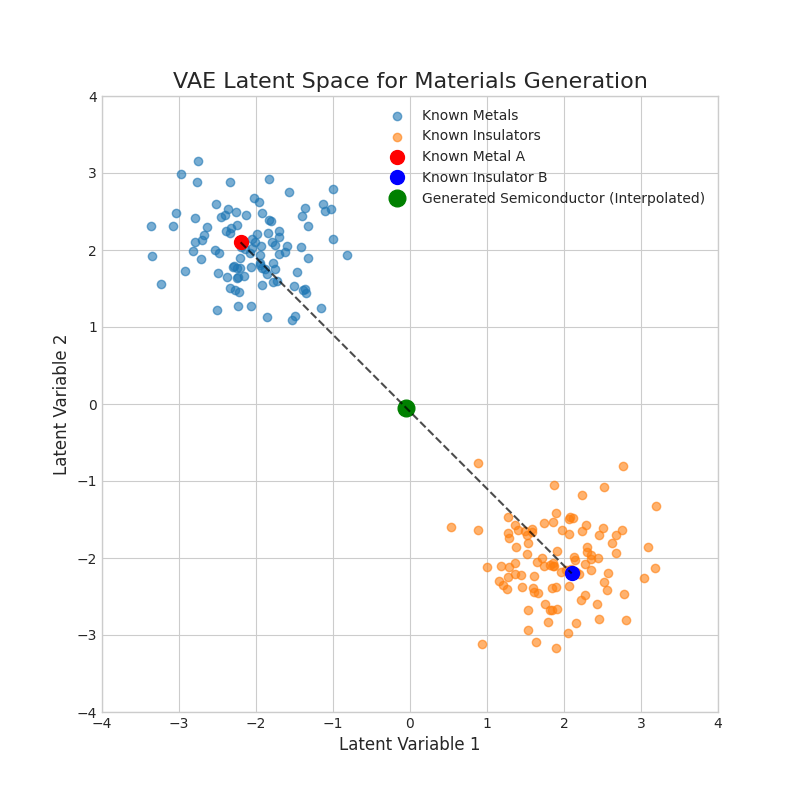
A generative model is trained on a vast database of existing materials. It learns a compressed, continuous "latent space" representation of these materials. To design a new material, one can sample a point in this latent space and decode it to generate a novel crystal structure. By linking properties to coordinates in this latent space, we can intelligently search for new materials.
Simplified Python Example (Conceptual):
This code conceptually illustrates how a VAE might be used for inverse design. We'll use dummy data for simplicity, but the logic remains the same. The key idea is to have an encoder that maps a material to the latent space, and a decoder that maps a point in the latent space back to a material.
import torch
import torch.nn as nn
import torch.nn.functional as F

# ─────────────────────────────────────────────
# Corresponding formula:
#   L(θ,φ;x) = E[log p_θ(x|z)] - KL(q_φ(z|x) || p(z))
#            = Reconstruction Loss - KL Divergence
# ─────────────────────────────────────────────

class VAE(nn.Module):
    def __init__(self, input_dim=2, latent_dim=1):
        super().__init__()
        # Encoder: q_φ(z|x) → outputs the mean μ and log variance log σ²
        self.fc_mu     = nn.Linear(input_dim, latent_dim)
        self.fc_logvar = nn.Linear(input_dim, latent_dim)
        # Decoder: p_θ(x|z) → reconstruct x from z
        self.fc_decode = nn.Linear(latent_dim, input_dim)

    def encode(self, x):
        mu     = self.fc_mu(x)
        logvar = self.fc_logvar(x)
        return mu, logvar

    def reparameterize(self, mu, logvar):
        # Reparameterization trick: z = μ + ε·σ, where ε ~ N(0,1)
        # This is the key that allows backpropagation in VAE;
        # this step was completely missing in the original description
        std = torch.exp(0.5 * logvar)
        eps = torch.randn_like(std)
        return mu + eps * std

    def decode(self, z):
        return self.fc_decode(z)

    def forward(self, x):
        mu, logvar = self.encode(x)
        z          = self.reparameterize(mu, logvar)
        x_recon    = self.decode(z)
        return x_recon, mu, logvar


def vae_loss(x, x_recon, mu, logvar):
    # ① Reconstruction Loss: corresponds to E[log p_θ(x|z)] in the formula
    recon_loss = F.mse_loss(x_recon, x, reduction='sum')

    # ② KL Divergence: corresponds to KL(q_φ(z|x) || N(0,I)) in the formula
    # Closed-form: -0.5 * Σ(1 + log σ² - μ² - σ²)
    kl_loss = -0.5 * torch.sum(1 + logvar - mu.pow(2) - logvar.exp())

    return recon_loss + kl_loss


# ── Example training loop ─────────────────────
# Simulated materials data: [lattice parameter, band gap]
data = torch.tensor([[3.5, 1.2], [4.1, 0.8], [3.8, 1.5],
                     [5.2, 0.1], [4.5, 1.0], [3.2, 1.8]], dtype=torch.float32)

model     = VAE(input_dim=2, latent_dim=1)
optimizer = torch.optim.Adam(model.parameters(), lr=1e-2)

for epoch in range(300):
    x_recon, mu, logvar = model(data)
    loss = vae_loss(data, x_recon, mu, logvar)
    optimizer.zero_grad()
    loss.backward()
    optimizer.step()

print(f"Final loss: {loss.item():.4f}")

# ── Inverse design: sample in the latent space to generate new materials ──
with torch.no_grad():
    z_sample    = torch.randn(5, 1)          # Sample from N(0,1)
    new_material = model.decode(z_sample)
    print("Generated materials (latent space sampling):")
    print(new_material)
2. Physics-Informed Neural Networks (PINNs)
PINNs are neural networks that are trained to respect the fundamental laws of physics. In materials science, this means that instead of just learning from data, the model's predictions must also satisfy governing physical equations, like those of quantum mechanics or thermodynamics.
Concept:
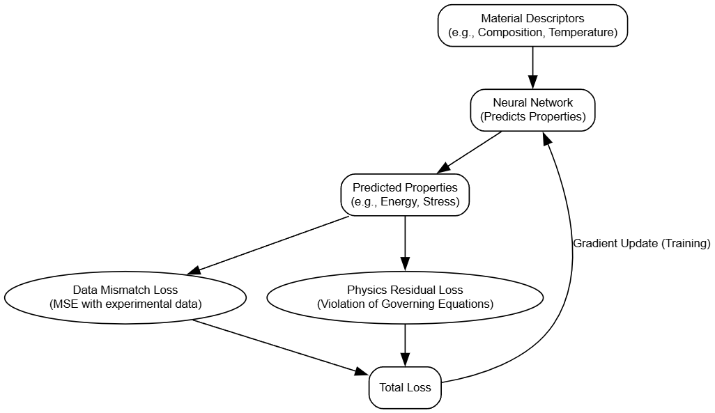
The loss function of a PINN has two components: a data-driven loss (how well it fits the observed data) and a physics-based loss (how well it satisfies the governing equations). This makes PINNs particularly powerful when experimental data is scarce, as the physics-based loss regularizes the model and prevents it from making physically implausible predictions.
Diagram: PINN Architecture
Here’s a diagram illustrating the concept of a PINN.

3. Graph Neural Networks (GNNs) for Crystal Structures
Crystal structures are naturally represented as graphs, where atoms are nodes and bonds are edges. GNNs are a class of neural networks specifically designed to operate on graph-structured data. They have become a cornerstone of modern materials modeling because they can learn features directly from the atomic structure.
Concept:
GNNs work by passing "messages" between connected nodes (atoms) in the graph. Through successive layers of message passing, each atom's representation is updated to include information about its local chemical environment. This allows the GNN to learn a holistic representation of the entire crystal structure, which can then be used to predict its properties.
Simplified Python Example (Conceptual):
This code demonstrates the core idea of message passing in a GNN. We'll use a simple "molecule" (a water molecule) as our graph.
import torch
import torch.nn as nn
import torch.nn.functional as F

# ─────────────────────────────────────────────
# Corresponding formula:
#   h_i^(l+1) = σ( W^(l) · ( h_i^(l) + Σ_{j∈N(i)} h_j^(l) ) )
# ─────────────────────────────────────────────

class GNNLayer(nn.Module):
    """Single GNN layer implementing one round of message passing"""
    def __init__(self, in_dim, out_dim):
        super().__init__()
        # W^(l): learnable weight matrix
        # The original text used a fixed random value;
        # here it is correctly defined as a trainable parameter
        self.W = nn.Linear(in_dim, out_dim, bias=False)

    def forward(self, H, adj):
        """
        H   : (N, in_dim)  current node feature matrix
        adj : (N, N)       adjacency matrix
        """
        # Aggregation: Σ_{j∈N(i)} h_j^(l)
        # Matrix form: adj @ H
        # Row i becomes the sum of features of all neighbors of node i
        neighbor_sum = adj @ H

        # Update: h_i + aggregated neighbor features
        aggregated = H + neighbor_sum

        # Linear transformation W^(l) followed by nonlinearity σ (ReLU)
        # The original code missed this step, which does not match the σ in the formula
        return F.relu(self.W(aggregated))


class GNN(nn.Module):
    def __init__(self, in_dim=2, hidden_dim=4, out_dim=1):
        super().__init__()
        self.layer1 = GNNLayer(in_dim, hidden_dim)
        self.layer2 = GNNLayer(hidden_dim, hidden_dim)
        # Graph-level prediction:
        # average node features and map to the target property
        self.readout = nn.Linear(hidden_dim, out_dim)

    def forward(self, H, adj):
        H = self.layer1(H, adj)    # First round of message passing
        H = self.layer2(H, adj)    # Second round of message passing
        # Global mean pooling:
        # aggregate all atomic features into a crystal-level representation
        graph_repr = H.mean(dim=0, keepdim=True)
        return self.readout(graph_repr)


# ── Water molecule graph definition (consistent with original text) ──
# Node features: [atomic number, electronegativity] (simplified)
#   H1: [1, 2.2], O: [8, 3.4], H2: [1, 2.2]
H_init = torch.tensor([
    [1.0, 2.2],   # H1
    [8.0, 3.4],   # O
    [1.0, 2.2],   # H2
], dtype=torch.float32)

# Symmetric adjacency matrix (including self-loops to retain self-information)
adj = torch.tensor([
    [1, 1, 0],
    [1, 1, 1],
    [0, 1, 1],
], dtype=torch.float32)

# Target: predict a scalar property
# (e.g., formation energy; here a fictitious value is used for demonstration)
y_target = torch.tensor([[1.5]])

# ── Training ─────────────────────────────────────
model     = GNN(in_dim=2, hidden_dim=4, out_dim=1)
optimizer = torch.optim.Adam(model.parameters(), lr=1e-2)

for epoch in range(500):
    y_pred = model(H_init, adj)
    loss   = F.mse_loss(y_pred, y_target)
    optimizer.zero_grad()
    loss.backward()   # W is truly updated via gradients; in the original text W was never updated
    optimizer.step()

    if epoch % 100 == 0:
        print(f"Epoch {epoch:3d} | pred={y_pred.item():.4f} | loss={loss.item():.4f}")
These innovative modeling approaches are rapidly accelerating the pace of materials discovery and design. By combining the power of machine learning with fundamental physical principles, researchers can explore vast chemical spaces, predict material properties with increasing accuracy, and design novel materials with tailored functionalities.
Mathematical Principles in Machine Learning: Analysis and Visualisation
1. Generative Models: The Variational Autoencoder (VAE)
The magic of VAEs lies in how they structure their latent space. Unlike standard autoencoders, a VAE's latent space is continuous and probabilistic, which is perfect for generating new, unseen data. This is achieved by optimizing a special loss function called the Evidence Lower Bound, or ELBO.
Mathematical Formula:
The goal of a VAE is to maximize the likelihood of the data, which is often intractable. Instead, we maximize the ELBO, which is a lower bound on this likelihood. Maximizing the ELBO is equivalent to minimizing the VAE's loss function. The loss function is composed of two key terms:
$$ \mathcal{L}(\theta, \phi; \mathbf{x}) = \underbrace{\mathbb{E}_{q_{\phi}(\mathbf{z}|\mathbf{x})}[\log p_{\theta}(\mathbf{x}|\mathbf{z})]}_{\text{Reconstruction Loss}} - \underbrace{D_{KL}(q_{\phi}(\mathbf{z}|\mathbf{x}) || p(\mathbf{z}))}_{\text{KL Divergence (Regularization)}} $$
Reconstruction Loss
This term pushes the VAE to accurately reconstruct the input material $\mathbf{x}$ from its latent representation $\mathbf{z}$. It is the expected log-likelihood of the data given the latent variable. In practice, this often behaves like a Mean Squared Error for continuous data.
KL Divergence
This is the crucial regularization term. It measures how much the distribution learned by the encoder, $q_{\phi}(\mathbf{z}|\mathbf{x})$, deviates from a prior distribution, typically a standard normal distribution $p(\mathbf{z}) = \mathcal{N}(0, I)$. By minimizing this divergence, we force the latent space to be smooth and centered around the origin, which allows for meaningful interpolation to create novel materials.
Visualization: A Smooth Latent Space
A well-trained VAE creates a smooth latent space where similar materials are clustered together. We can then sample a point that lies between two known materials and decode it to generate a new material with hybrid properties. The Python code generates a plot illustrating this concept.

2. Physics-Informed Neural Networks (PINNs)
PINNs embed physical laws directly into the training of a neural network. This is done by adding a "physics loss" term to the standard data-driven loss. This term penalizes the network if its predictions violate a known governing differential equation.
Mathematical Formula
The total loss function for a PINN is a weighted sum of the data loss and the physics loss:
$$ \mathcal{L}_{Total} = \mathcal{L}_{Data} + \lambda \mathcal{L}_{Physics} $$
More detailed:
$ \mathcal{L}_{Data} = \frac{1}{N} \sum_{i=1}^{N} (u(x_i) - y_i)^2 $
This is the standard Mean Squared Error (MSE), where $u(x_i)$ is the neural network's prediction at data point $x_i$, and $y_i$ is the known experimental or simulation value.
$ \mathcal{L}_{Physics} = \frac{1}{M} \sum_{j=1}^{M} (f(\frac{\partial u}{\partial t}, \frac{\partial u}{\partial x}, \frac{\partial^2 u}{\partial x^2}, ...))^2 $
This is the physics residual. The function $f$ represents the governing PDE. For example, for the 1D heat equation, $f = \frac{\partial u}{\partial t} - \alpha \frac{\partial^2 u}{\partial x^2} = 0$. The network is penalized for any point where $f$ is not zero. The derivatives ($\frac{\partial u}{\partial t}$, etc.) are calculated efficiently using automatic differentiation.
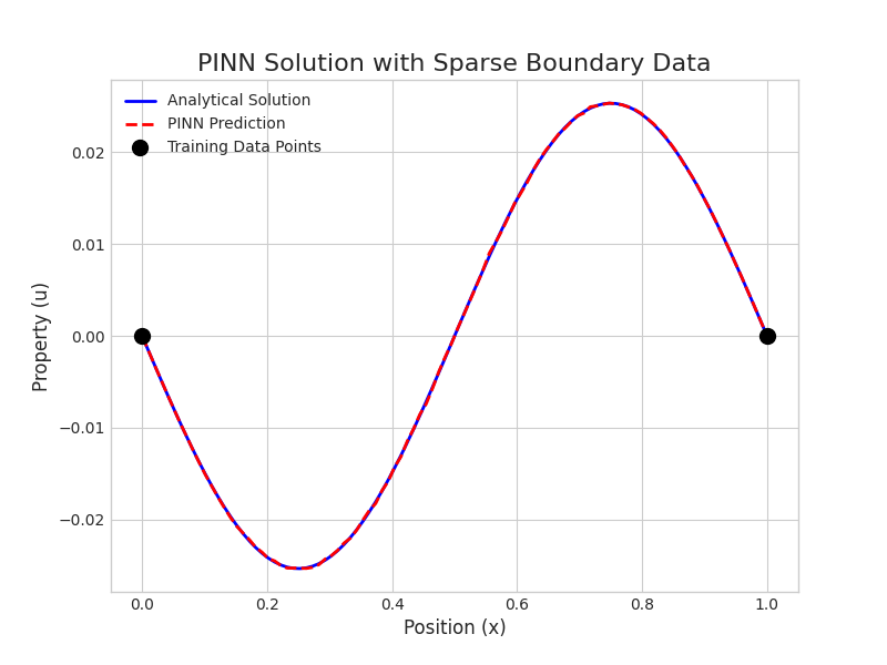
Visualization: Solving a PDE with Sparse Data
A key advantage of PINNs is their ability to find a solution in regions with no data. The code below trains a simple neural network to solve a steady-state equation with boundary conditions, showing how the model's adherence to the physical law fills in the gaps.

3. Graph Neural Networks (GNNs)
GNNs are ideal for modeling crystal structures because they operate directly on graph representations of atoms (nodes) and bonds (edges). The core operation is "message passing," where atoms iteratively update their feature representations based on information from their neighbors.
Mathematical Formula:
A common message-passing update rule for a node (atom) $i$ at layer $l+1$ can be expressed as:
$$ \mathbf{h}_i^{(l+1)} = \sigma \left( \mathbf{W}^{(l)} \cdot \left( \mathbf{h}_i^{(l)} + \sum_{j \in \mathcal{N}(i)} \mathbf{h}_j^{(l)} \right) \right) $$
- $\mathbf{h}_i^{(l+1)}$ is the new feature vector, or "embedding," for atom $i$.
- $\sigma$ is a non-linear activation function, like ReLU.
- $\mathbf{W}^{(l)}$ is a learnable weight matrix for layer $l$.
- $\mathbf{h}_i^{(l)}$ is the feature vector of atom $i$ from the previous layer.
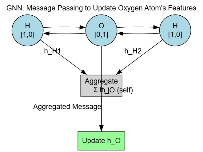
- $\sum_{j \in \mathcal{N}(i)} \mathbf{h}_j^{(l)}$ is the aggregation step, where atom $i$ sums the feature vectors of all its neighboring atoms $j$. This is how information about the local chemical environment is gathered.
After several rounds of message passing, the final node embeddings can be aggregated (e.g., by averaging) to produce a single feature vector for the entire crystal, which is then used to predict material properties.
Diagram: Message Passing in a GNN
This graph visualizes one step of message passing. The central Oxygen atom aggregates the feature vectors from its two Hydrogen neighbors to update its own representation, thus learning about its local environment.

I hope these mathematical elaborations and visualizations provide a clearer picture of how these cutting-edge models are revolutionizing materials science.
Ref.
- Wei, J., Chu, X., Sun, X.-Y., Xu, K., Deng, H.-X., Chen, J., Wei, Z. & Lei, M. (2019). Machine learning in materials science. InfoMat.
- Jain, A. (2024). Machine learning in materials research: Developments over the last decade. Curr. Opin. Solid State Mater. Sci.
- Chong, S. S., Ng, Y. S., Wang, H.-Q., & Zheng, J.-C. (2024). Advances of machine learning in materials science: Ideas and techniques. Front. Phys.
作者:GARFIELDTOM
邮箱:coolerxde@gt.ac.cn