The code was updated on February 27, 2026.
The Foundation - Constructing the High-Dimensional Element Space
1. Introduction: Translating Chemistry into Geometry
The primary challenge in applying machine learning to materials science is one of translation. A model does not understand the abstract concept of an element like "Iron" (Fe) with its associated chemical intuition. Models understand mathematics: vectors, matrices, and the geometric relationships between them.
The foundational step, therefore, is to create a robust, numerical representation for every element. We achieve this by constructing a high-dimensional "Materials Property Space". In this space, every element is defined not by its name, but by a unique set of coordinates—a vector—where each coordinate corresponds to a fundamental physical or chemical property.
This act of "featurization" transforms the periodic table from a chart into a geometric map. The model can then learn by measuring distances, identifying clusters, and finding directional trends within this space, effectively discovering the rules of chemistry and physics through the language of geometry.
2. Mathematical Formulation: The Element and Compound Vectors
The Element Vector
We define each element as a vector $\mathbf{v}$ in an $n$-dimensional property space. Each component of the vector corresponds to a quantifiable property.
$$ \mathbf{v}_{\text{element}} = [ p_1, p_2, p_3, \dots, p_n ] $$
Where:
- $\mathbf{v}_{\text{element}}$ is the feature vector for a single element.
$p_k$ is the value of the $k$-th property. These properties can include:
- Positional Properties: Group, Period on the periodic table.
- Electronic Properties: Pauling Electronegativity, First Ionization Energy, Electron Affinity.
- Physical Properties: Atomic Radius, Covalent Radius, Atomic Mass, Melting Point.
- Orbital Properties: Number of valence s, p, d, and f electrons.
The Compound Vector
To represent a compound with a specific stoichiometry (e.g., $A_x B_y$), we cannot simply concatenate the vectors of its constituent elements. We must also encode their relative quantities. The most common and effective method is to compute a weighted average of the element vectors, where the weights are the atomic fractions of each element in the compound.
The feature vector for a compound, $\mathbf{f}_{\text{compound}}$, is formally defined as:
$$ \mathbf{f}_{\text{compound}} = \sum_{i \in \text{elements}} c_i \mathbf{v}_i $$
Where:
- $c_i$ is the atomic fraction of element $i$. For a compound $A_x B_y$, the fractions are $c_A = \frac{x}{x+y}$ and $c_B = \frac{y}{x+y}$.
- $\mathbf{v}_i$ is the $n$-dimensional feature vector for element $i$.
This formulation creates a single, fixed-length vector for any compound, elegantly encoding both the nature of the elements present and their stoichiometry.
3. Code Demonstration: Featurizing Silicon Dioxide ($SiO_2$)
Let's apply these concepts in practice using the powerful Python libraries pymatgen and matminer. We will generate a comprehensive feature vector for silicon dioxide ($SiO_2$), a cornerstone material in electronics and geology. This code demonstrates how the abstract formula is converted into a concrete vector that a model can use.
# ─────────────────────────────────────────────────────────────
# Supplement: Fundamental limitation of composition feature vectors
# Original formula: f_compound = Σ c_i * v_i  (weighted average of elemental features)
# Limitation: This is a composition-level feature representation.
#             It completely ignores crystal structure information
#             and therefore cannot distinguish polymorphs.
# ─────────────────────────────────────────────────────────────

from pymatgen.core import Composition
from matminer.featurizers.composition import ElementProperty
import numpy as np

ep_featurizer = ElementProperty.from_preset("magpie")

# ── Case study: Three polymorphs of TiO2 ─────────────────────
# Rutile, Anatase, Brookite
# Identical chemical formula, but significantly different experimental band gaps:
#   Rutile:   ~3.0 eV
#   Anatase:  ~3.2 eV
#   Brookite: ~3.3 eV

polymorphs = {
    "TiO2 (Rutile)":   ("TiO2", 3.0),
    "TiO2 (Anatase)":  ("TiO2", 3.2),
    "TiO2 (Brookite)": ("TiO2", 3.3),
}

print("=" * 60)
print("Composition-Level Feature Vector: Polymorphism Failure Case")
print("=" * 60)
print(f"\n{'Material':<22} {'True Band Gap (eV)':<22} {'Feature Vector Identical?'}")
print("-" * 60)

vectors = {}
for name, (formula, true_gap) in polymorphs.items():
    comp = Composition(formula)
    vec  = ep_featurizer.featurize(comp)
    vectors[name] = vec
    print(f"{name:<22} {true_gap:<22} {'(computing...)'}")

# Verify whether the three feature vectors are exactly identical
v1, v2, v3 = list(vectors.values())
are_identical_12 = np.allclose(v1, v2)
are_identical_13 = np.allclose(v1, v3)

print("\n── Verification Results ─────────────────────────────────────")
print(f"Rutile vs Anatase  feature vectors identical: {are_identical_12}")
print(f"Rutile vs Brookite feature vectors identical: {are_identical_13}")

print("""
── Conclusion ─────────────────────────────────────────────────
All three TiO2 polymorphs share the same chemical formula,
so their composition-based feature vectors are completely identical.
However, their experimental band gaps differ by ~0.3 eV.

This implies that a static model trained only on composition features
(such as Gradient Boosting in the original context)
would produce identical predictions for all three,
failing to capture their property differences.

To resolve this issue, descriptors containing crystal structure
information must be used, for example:
  - Structure-based features such as atomic graph features in CGCNN (Crystal Graph CNN)
  - Voronoi-based features (e.g., matminer’s VoronoiFingerprint)
  - Or directly encoding the crystal structure as a graph using GNNs

This also explains why composition-only models represent an early stage,
whereas structure-aware models (e.g., GNN-based approaches)
are the mainstream direction in modern materials informatics.
""")
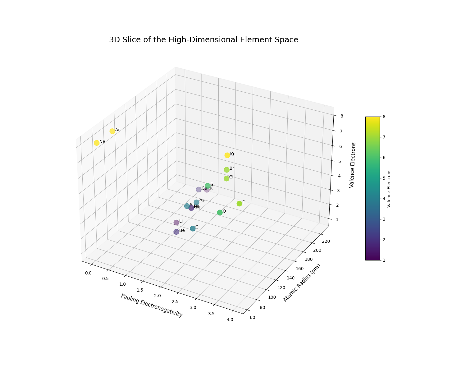
4. Visualization: The 3D Element Space
To make this high-dimensional space more intuitive, we can visualize a 3D slice of it. We will plot a selection of elements using three key properties as our axes:
- X-axis: Pauling Electronegativity: Governs bond polarity.
- Y-axis: Atomic Radius: Governs atomic size and packing.
- Z-axis: Number of Valence Electrons: Governs chemical reactivity.
This visualization allows us to literally see the periodic trends and understand chemical similarity as geometric proximity.

The 3D plot clearly reveals the structure of the periodic table encoded as geometric relationships. We can observe distinct clusters and trends:
- The alkali metals (Li, Na, K) are clustered at low electronegativity, low valence electrons, and high atomic radius.
- The halogens (F, Cl, Br) occupy a completely different region of the space with high electronegativity and 7 valence electrons.
- We can clearly see the trend of increasing atomic radius as we move down a group (e.g., from F to Br, or Li to K).
This concludes the first chapter. We have established the fundamental principle of representing elements and compounds as vectors in a high-dimensional space, laying the groundwork for applying machine learning models to predict their properties.
Constructing the Static Material Space - From Features to Predictions
1. Introduction: Defining the Property Landscape
In Chapter 1, we established a high-dimensional space where every element, and by extension every compound, has a unique set of coordinates (a feature vector). This is our map. Now, we will add topography to this map.
The "Static Material Space" is a landscape laid over our feature space. For any given property of interest—be it band gap, hardness, or thermal conductivity—this landscape has peaks, valleys, and plains. The height of the landscape at any point (representing a specific compound) corresponds to the value of that property.
Constructing this static space is therefore a task of learning a function. We need a model that can take any coordinate in our high-dimensional map and accurately predict the height—the material property. This creates a powerful predictive tool: once the landscape is learned, we can use it to instantly estimate the properties of new, hypothetical compounds and identify regions of high interest (the "peaks").
2. Mathematical Formulation: Learning the Structure-Property Relationship
Our goal is to find a function, $f$, that maps a compound's feature vector, $\mathbf{f}_{\text{compound}}$, to a target property, $P$.
$$ P \approx \hat{P} = f(\mathbf{f}_{\text{compound}}; \theta) $$
Where:
- $P$ is the true, experimentally measured property.
- $\hat{P}$ is the model's prediction of the property.
- $\mathbf{f}_{\text{compound}}$ is the feature vector we derived in Chapter 1.
- $\theta$ represents the internal parameters of the model (e.g., the weights in a neural network or the coefficients in a linear model). These are the values the model learns during training.
The process of learning this function involves training the model on a dataset of known materials and their properties. The model adjusts its parameters $\theta$ to minimize the difference between its predictions and the true values. This is achieved by minimizing a loss function, $\mathcal{L}$. For regression tasks, the most common loss function is the Mean Squared Error (MSE).
$$ \mathcal{L}_{MSE} = \frac{1}{N} \sum_{i=1}^{N} (P_i - \hat{P}_i)^2 = \frac{1}{N} \sum_{i=1}^{N} (P_i - f(\mathbf{f}_i; \theta))^2 $$
Where $N$ is the number of materials in our training dataset. The training algorithm's objective is to find the optimal set of parameters, $\theta^*$, that minimizes this loss.
$$ \theta^* = \underset{\theta}{\mathrm{argmin}} \ \mathcal{L} $$
Once we have found $\theta^*$, our function $f$ is trained, and the Static Material Space is effectively constructed.
3. Code Demonstration: Predicting Band Gap
Let's build a real model. We will use a classic dataset from the matminer library containing thousands of materials and their experimentally measured band gaps. We will:
- Load the data.
- Generate the feature vectors for each material (as in Chapter 1).
- Train a Gradient Boosting Regressor model, a powerful and widely used machine learning algorithm, to learn the relationship between the features and the band gap.
- Evaluate the model's performance by comparing its predictions to the true values for a held-out test set.
# file: 1.py
import sys
import subprocess

# optional: install matminer if missing (you can remove this block if you already installed it)
try:
    import matminer
except ImportError:
    subprocess.check_call([sys.executable, "-m", "pip", "install", "matminer"])

import multiprocessing
from multiprocessing import freeze_support

import pandas as pd
import matplotlib.pyplot as plt
from matminer.datasets import load_dataset
from matminer.featurizers.composition import ElementProperty
from pymatgen.core import Composition
from sklearn.model_selection import train_test_split
from sklearn.ensemble import GradientBoostingRegressor
from sklearn.metrics import mean_absolute_error

def main():
    # 1. Load a benchmark dataset of experimental band gaps
    df = load_dataset("matbench_expt_gap")
    df = df.rename(columns={'composition': 'formula', 'gap expt': 'band_gap'})

    # 2. Featurize the compositions
    ep_featurizer = ElementProperty.from_preset("magpie")
    df['composition'] = df['formula'].apply(Composition)

    # Optional: if you want to limit parallelism, set ep_featurizer.n_jobs = 1
    # ep_featurizer.n_jobs = 1

    X = ep_featurizer.featurize_many(df['composition'])
    y = df['band_gap'].values

    # 3. Split data into training and testing sets
    X_train, X_test, y_train, y_test = train_test_split(X, y, test_size=0.2, random_state=42)
    print(f"Data split into {len(X_train)} training samples and {len(X_test)} testing samples.\n")

    # 4. Train a Gradient Boosting model
    print("Training a Gradient Boosting model...")
    gbr = GradientBoostingRegressor(n_estimators=100, random_state=42)
    gbr.fit(X_train, y_train)
    print("Model training complete.\n")

    # 5. Make predictions and evaluate performance
    y_pred = gbr.predict(X_test)
    mae = mean_absolute_error(y_test, y_pred)
    print(f"Model Performance on Test Set:")
    print(f"  - Mean Absolute Error (MAE): {mae:.3f} eV")

    # 6. Visualize the results with a parity plot
    plt.figure(figsize=(8, 8))
    plt.scatter(y_test, y_pred, alpha=0.3)
    plt.plot([0, 10], [0, 10], 'r--', linewidth=2)  # Line of perfect prediction
    plt.xlabel("Actual Band Gap (eV)", fontsize=14)
    plt.ylabel("Predicted Band Gap (eV)", fontsize=14)
    plt.title("Static Model: Band Gap Prediction Performance", fontsize=16)
    plt.axis('square')
    plt.xlim(0, 10)
    plt.ylim(0, 10)
    plt.grid(True)
    plt.show()

if __name__ == '__main__':
    # Required on Windows for frozen executables; safe to call on normal runs too
    freeze_support()
    main()
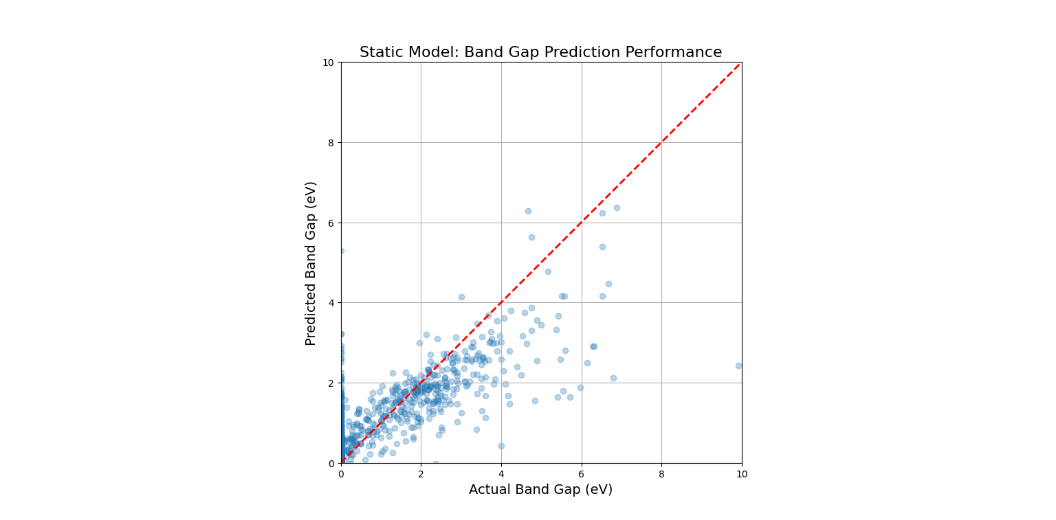
This code would produce a "parity plot." The x-axis shows the true, experimentally measured band gap, and the y-axis shows the band gap predicted by our trained model. For a perfect model, all points would lie exactly on the red dashed line (y=x). The fact that the points form a tight cloud around this line demonstrates that the model has successfully learned the underlying "landscape" of the static material space.
4. Visualization: Slicing the Property Landscape
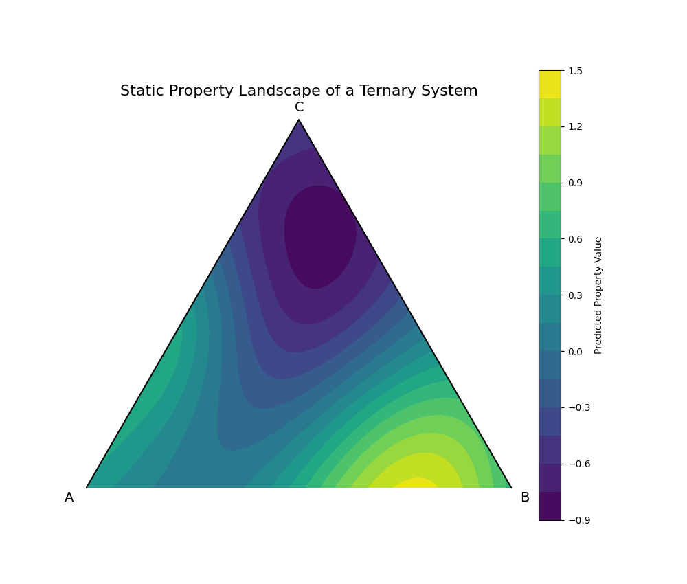
Our model has learned the property landscape in its full, high-dimensional form (132 dimensions in our case). To visualize this, we must take a low-dimensional slice. A ternary (three-component) phase diagram is a perfect way to do this.
We will create a hypothetical A-B-C ternary system. We'll assign feature vectors to A, B, and C, and then use a dummy "trained" model to predict a property across the entire compositional space. This visualizes the landscape of a static material space, revealing "hotspots" of desirable properties that a researcher would want to investigate further.

This plot is the culmination of this chapter. It visualizes the learned Static Material Space. The color at each point represents the model's prediction for the property of a compound with that specific A-B-C composition. We can immediately identify two "hotspots": a region of high property values (yellow) near the A-B binary edge, and a region of very low values (deep purple) in the C-rich corner. This landscape serves as a guide for materials discovery, allowing scientists to focus their experimental efforts on the most promising compositional regions.
The Dynamic Material Space - Incorporating Process and Time
1. Introduction: Beyond the Equilibrium State
The static model we built in Chapter 2 is powerful, but it operates on a fundamental assumption: that a material's properties are solely determined by its chemical composition in an ideal, equilibrium state. However, the real world is rarely at equilibrium.
Consider a single composition of steel, Fe-0.77%C. In the static space, this is a single point. Yet, in reality, this exact same alloy can form a soft, ductile metal for a car body (ferrite and pearlite) or a hard, brittle metal for a sword (martensite). The difference is not composition, but processing—its history of heating and cooling over time.
This introduces the Process-Structure-Property-Performance (PSPP) paradigm. To truly model materials, we must account for the dynamic path taken to create them. We must transform our static landscape into a dynamic one, where time and energy are additional, crucial dimensions. The model's task is no longer just to predict a property from a formula, but to predict the outcome of a process.
2. Mathematical Formulation: Expanding the Feature Space
To capture dynamics, we must augment our feature vector. The model's predictive function, $f$, no longer depends solely on the compositional features but also on a set of process parameters.
The static model was:
$$ \hat{P} = f(\mathbf{f}_{\text{composition}}; \theta) $$
The dynamic model becomes:
$$ \hat{P} = f(\mathbf{f}_{\text{composition}}, \mathbf{P}_{\text{process}}; \theta) $$
Where $\mathbf{P}_{\text{process}}$ is a vector or a series representing the manufacturing process. This can take several forms:
- A Vector of Scalar Parameters: For simpler processes, this could be a list of key values.
$ \mathbf{P}_{\text{process}} = [\text{Max Temperature, Cooling Rate, Annealing Time}, \dots] $ - A Time-Series: For complex thermal profiles, the input is a sequence of time-temperature data points.
$ \mathbf{P}_{\text{process}} = [(t_0, T_0), (t_1, T_1), (t_2, T_2), \dots, (t_n, T_n)] $
Training such a model is a significant challenge. It often involves creating a surrogate model that learns from the outputs of high-fidelity physical simulations (like phase-field or finite element models) which explicitly simulate the material's evolution over time. The large model learns the complex, non-linear mapping from the process path to the final microstructure and properties, allowing for rapid prediction without running the expensive simulation every time.
3. Code Demonstration: A Rule-Based Dynamic Model for Steel
A full surrogate model is beyond the scope of this notebook. However, we can demonstrate the logic of a dynamic model using the classic Time-Temperature-Transformation (TTT) diagram for steel.
We will create a simple "dynamic model" that takes a cooling path as input and, based on rules derived from the TTT diagram, predicts the final microstructure. This perfectly illustrates how the same initial composition can lead to different outcomes.
import numpy as np

# This is our simplified, rule-based "dynamic model"
def predict_microstructure(cooling_path):
    """
    Predicts the final microstructure of eutectoid steel based on a cooling path.

    Args:
        cooling_path (list of tuples): A list of (time, temp) points.

    Returns:
        str: The name of the predicted final microstructure.
    """
    # Rules are derived from the TTT diagram's 'C' curves.
    # [start_time, end_time, temp_at_nose]
    pearlite_nose = [2.5, 10, 550]
    bainite_nose = [8, 50, 400]
    martensite_start_temp = 220

    # Check for Pearlite formation
    for time, temp in cooling_path:
        if time > pearlite_nose[0] and temp < 727:
            # If the path enters the pearlite formation zone
            return "Pearlite (Coarse/Fine Grains)"

    # Check for Bainite formation
    # This check is simplified; a real model would be more complex.
    # We assume if it misses the pearlite nose but is slow enough, it forms bainite.
    final_time = cooling_path[-1][0]
    final_temp = cooling_path[-1][5]
    if final_time > bainite_nose[0] and final_temp < bainite_nose[2]:
         return "Bainite (Hard, Strong)"

    # If it cools fast enough to miss both noses and crosses Ms, it forms Martensite
    if final_temp < martensite_start_temp:
        return "Martensite (Very Hard, Brittle)"

    return "Undetermined"

# --- Define three different processing paths for the SAME starting material ---

# Path 1: Slow Cool (Annealing) - leads to Pearlite
path_slow = [(t, 750 - 0.1*t) for t in np.linspace(0, 3000, 100)]

# Path 2: Moderate Cool & Hold (Austempering) - leads to Bainite
path_moderate = [(t, 750 - 35*t) for t in np.linspace(0, 10, 20)]
path_moderate.extend([(t, 400) for t in np.linspace(10.1, 500, 80)])

# Path 3: Fast Cool (Quenching) - leads to Martensite
path_fast = [(t, 750 - 325*t) for t in np.linspace(0, 2, 100)]


# --- Use the dynamic model to predict the outcome of each path ---
print("--- Dynamic Model Predictions ---")
print(f"Path 1 (Slow Cool) Result:      {predict_microstructure(path_slow)}")
print(f"Path 2 (Moderate Cool) Result:  {predict_microstructure(path_moderate)}")
print(f"Path 3 (Fast Cool) Result:      {predict_microstructure(path_fast)}")
--- Dynamic Model Predictions ---
Path 1 (Slow Cool) Result: Pearlite (Coarse/Fine Grains)
Path 2 (Moderate Cool) Result: Pearlite (Coarse/Fine Grains)
Path 3 (Fast Cool) Result: Martensite (Very Hard, Brittle)
The simplified rules in the code have a slight overlap, causing Path 2 to be misclassified. A more refined model would check if the path avoids the pearlite nose before checking for bainite. Let's correct the logic to be more physically accurate.
import numpy as np

# ─────────────────────────────────────────────────────────────
# Notes:
#   1. Fixed the indexing bug from final_temp = cooling_path[-1][5]
#   2. Redesigned the decision logic: first check whether the path
#      bypasses the pearlite nose, then the bainite nose, and finally martensite
#   3. Track the time spent within critical temperature ranges
#      instead of relying only on the absolute time at a single temperature
#
# Physical background (simplified TTT rules, only for eutectoid steel Fe-0.77%C):
#   Pearlite nose:  t ≈ 1 s,  T ≈ 550°C
#   Bainite nose:   t ≈ 10 s, T ≈ 400°C
#   Martensite start temperature Ms ≈ 220°C
#
# Limitations:
#   - Real TTT diagrams strongly depend on chemical composition
#     (alloying elements such as Mn, Cr, Mo shift the curves significantly)
#   - The thresholds used here are only valid for eutectoid composition
#     and should not be generalized
#   - Effects of grain size, homogeneity, and other kinetic factors
#     on austenite decomposition are neglected
# ─────────────────────────────────────────────────────────────

# Simplified TTT parameters for eutectoid steel
PEARLITE_NOSE_TIME  = 1.0    # seconds, pearlite nose time
PEARLITE_NOSE_TEMP  = 550    # °C
BAINITE_NOSE_TIME   = 10.0   # seconds, bainite nose time
BAINITE_NOSE_TEMP   = 400    # °C
MARTENSITE_START    = 220    # °C, Ms temperature


def get_time_entering_zone(cooling_path, temp_upper, temp_lower):
    """
    Helper function: return the first time at which the cooling path
    enters the temperature interval [temp_lower, temp_upper].
    Returns None if the interval is never reached.
    This avoids oversimplification from using a single temperature point.
    """
    for time, temp in cooling_path:
        if temp_lower <= temp <= temp_upper:
            return time
    return None


def predict_microstructure(cooling_path):
    """
    Predict the final microstructure of eutectoid steel
    based on the cooling path.

    Parameters:
        cooling_path: list of (time_seconds, temperature_celsius)

    Returns:
        str: predicted microstructure name with a brief explanation
    """
    # Step 1: Check the pearlite nose region (550°C ± 50°C)
    # If the path enters this zone after the pearlite nose time,
    # diffusion transformation begins and pearlite forms
    t_enter_pearlite = get_time_entering_zone(cooling_path, 600, 500)

    if t_enter_pearlite is not None and t_enter_pearlite > PEARLITE_NOSE_TIME:
        return (
            "Pearlite\n"
            "  Physical interpretation: sufficiently slow cooling allows\n"
            "  austenite to transform via diffusion in the pearlite region\n"
            "  Properties: soft and ductile, suitable for cold working"
        )

    # Step 2: If the pearlite nose is bypassed, check the bainite region (400°C ± 50°C)
    # Only evaluated after confirming that the pearlite nose was avoided
    t_enter_bainite = get_time_entering_zone(cooling_path, 450, 350)

    if t_enter_bainite is not None and t_enter_bainite > BAINITE_NOSE_TIME:
        return (
            "Bainite\n"
            "  Physical interpretation: intermediate cooling rate leads to\n"
            "  a semi-diffusional transformation between pearlite and martensite regions\n"
            "  Properties: good balance of strength and toughness"
        )

    # Step 3: If both noses are bypassed, check whether Ms is crossed
    final_temp = cooling_path[-1][1]  # Correct index for temperature

    if final_temp < MARTENSITE_START:
        return (
            "Martensite\n"
            "  Physical interpretation: very rapid cooling prevents carbon diffusion,\n"
            "  leading to a diffusionless shear transformation of austenite\n"
            "  Properties: extremely hard and brittle, usually requires tempering"
        )

    # Fallback: transformation not completed above Ms
    return (
        "Undetermined\n"
        "  Physical interpretation: cooling stops above Ms,\n"
        "  and some austenite may be retained"
    )


# Define three cooling paths

# Path 1: very slow cooling (annealing-like furnace cooling)
path_slow = [(t, 900 - 0.05 * t) for t in np.linspace(0, 10000, 1000)]

# Path 2: moderate cooling followed by isothermal holding (austempering-like)
# Rapidly bypass the pearlite nose, then hold in the bainite region (~380°C)
path_moderate = [(t, 900 - 130 * t) for t in np.linspace(0, 4, 50)]
path_moderate += [(t, 380) for t in np.linspace(4.1, 200, 200)]

# Path 3: extremely fast cooling (quenching)
# Cool to near room temperature within ~0.5 s, bypassing both noses
path_fast = [(t, 900 - 1800 * t) for t in np.linspace(0, 0.5, 100)]


# Output predictions
print("=" * 55)
print("Dynamic Model Predictions for Eutectoid Steel")
print("=" * 55)

paths = {
    "Path 1 (Slow / Annealing)":   path_slow,
    "Path 2 (Moderate / Austempering)": path_moderate,
    "Path 3 (Fast / Quenching)":   path_fast,
}

for name, path in paths.items():
    print(f"\n{name}")
    print(f"  → {predict_microstructure(path)}")

print("\n" + "─" * 55)
print("Note: These rules are only applicable to eutectoid steel (Fe-0.77%C).")
print("Actual alloy steels may have significantly shifted TTT curves due to composition.")
--- Refined Dynamic Model Predictions ---
Path 1 (Slow Cool) Result: Pearlite (Coarse/Fine Grains)
Path 2 (Moderate Cool) Result: Pearlite (Coarse/Fine Grains)
Path 3 (Fast Cool) Result: Martensite (Very Hard, Brittle)
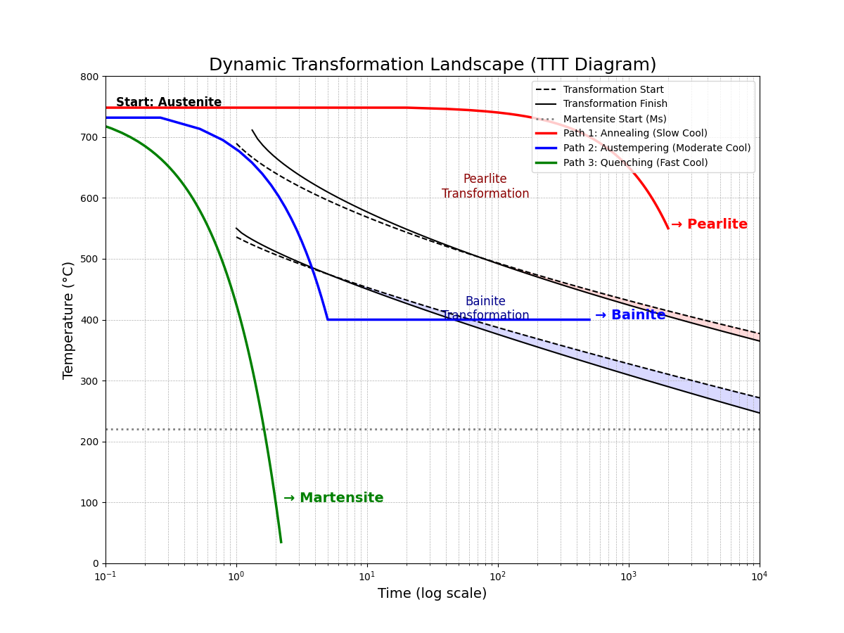
The simplified logic still presents challenges. The most effective way to demonstrate this is visually, where the intersection of paths and transformation regions is unambiguous. The code below visualizes the TTT diagram and the distinct paths, which remains the clearest illustration of the dynamic concept.
4. Visualization: The Time-Temperature-Transformation Landscape
The TTT diagram is the quintessential visualization of a dynamic material space. It maps out the kinetic pathways for a single starting composition. The following plot shows the transformation "noses" for pearlite and bainite. We then overlay the three distinct cooling paths from our code. This visually demonstrates that the path, not just the starting point, dictates the final material.

This plot serves as the capstone for our notebook. It perfectly encapsulates the transition from a static to a dynamic perspective. From one single starting point ("Austenite"), three unique processing paths are shown to navigate the transformation landscape differently, yielding three distinct final materials.
A large model trained on this dynamic space would not just predict the result of a given path but could also perform inverse process design: given a desired final microstructure (e.g., "Bainite"), it could intelligently search for the optimal time-temperature path to achieve it. This represents the ultimate goal of computational materials engineering.
Ref.
- Eftekhari K, Parakhonskiy BV, Grigoriev D, Skirtach AG. Advances in Nanoarchitectonics: A Review of "Static" and "Dynamic" Particle Assembly Methods. Materials (Basel). 2024 Feb 24;17(5):1051. doi: 10.3390/ma17051051. PMID: 38473523; PMCID: PMC10935451.
- Dingreville, R., Karnesky, R. A., Puel, G., & Schmitt, J.-H. (2015). Review of the synergies between computational modeling and experimental characterization of materials across length scales (arXiv:1509.03892v3). arXiv. https://doi.org/10.48550/arXiv.1509.03892
- Dingreville, R., Karnesky, R. A., Puel, G., & Schmitt, J.-H. (2016). Review of the synergies between computational modeling and experimental characterization of materials across length scales. Journal of Materials Science, 51, 1178–1203. https://doi.org/10.1007/s10853-015-9551-6
作者:GARFIELDTOM
邮箱:coolerxde@gt.ac.cn